Overview
This script demonstrates how to:
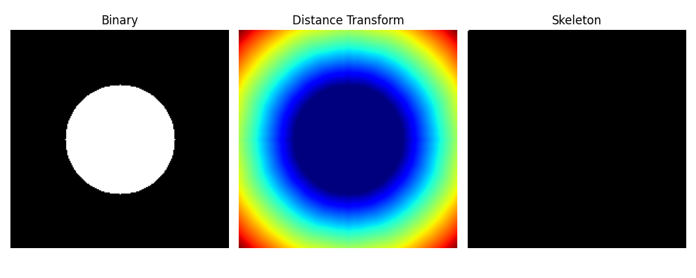
Generate a binary image with a simple shape.
Perform a distance transform to calculate the distance from each foreground pixel to the nearest background pixel.
Extract a basic “skeleton” by selecting the point(s) with the maximum distance.
Visualize the result using Matplotlib.
It uses OpenCV’s cv2.distanceTransform() to compute a Euclidean distance map and highlights the geometric center of the object, which corresponds to the furthest point from the boundary.
import cv2
import numpy as np
import matplotlib.pyplot as plt

# 1. Create a binary image
img = np.zeros((200, 200), dtype=np.uint8)
cv2.circle(img, (100, 100), 50, 255, -1) # Draw a white circle on black background

# 2. Prepare binary image for distance transform
binary = cv2.bitwise_not(img) # Uncomment this if your object is black on white background
#binary = img.copy() # Use the original binary image (white object on black background)

# 3. Apply distance transform
dist = cv2.distanceTransform(binary, cv2.DIST_L2, 5)

# 4. Extract skeleton (only the points with maximum distance)
skeleton = (dist == dist.max()).astype(np.uint8) * 255

# 5. Visualization using Matplotlib
plt.figure(figsize=(10, 4))

plt.subplot(1, 3, 1)
plt.title("Binary")
plt.imshow(img, cmap='gray')
plt.axis('off')

plt.subplot(1, 3, 2)
plt.title("Distance Transform")
plt.imshow(dist, cmap='jet')
plt.axis('off')

plt.subplot(1, 3, 3)
plt.title("Skeleton")
plt.imshow(skeleton, cmap='gray')
plt.axis('off')

plt.tight_layout()
plt.show()
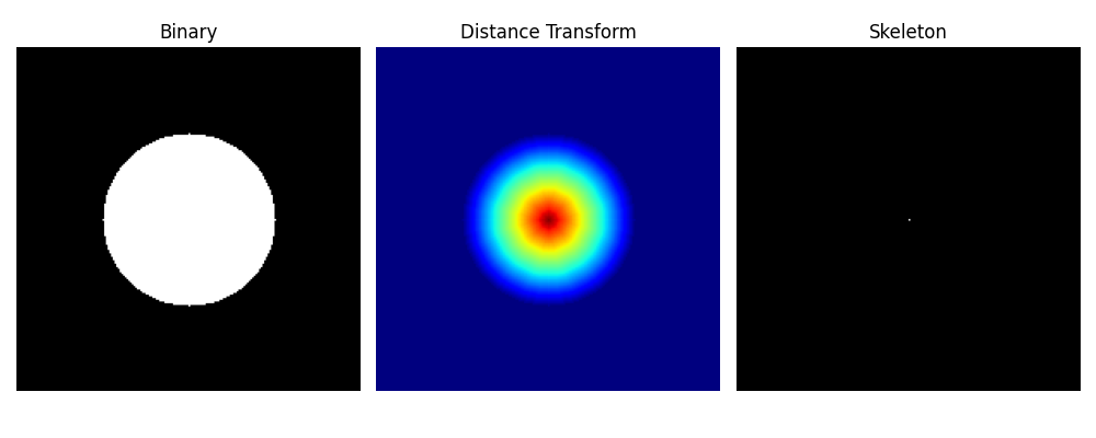
# Understanding cv2.distanceTransform()
The function cv2.distanceTransform() calculates the distance from each foreground pixel (non-zero) to the nearest background pixel (zero).
# Why do we sometimes invert the image?
The function expects a binary image where:
White (255) = foreground (object)
Black (0) = background
If your object is black on a white background (i.e., black = object, white = background), you need to invert the image using cv2.bitwise_not().
# Your understanding:
“The distance from a white pixel to the nearest black pixel”
→ This is correct, as long as:
White = object (foreground)
Black = background
# Summary:
If your image has a black object on a white background, invert it before using cv2.distanceTransform().
If your image already has a white object on a black background, you can use it directly.
import cv2
import numpy as np
import matplotlib.pyplot as plt
# 1. Create a binary image with a white filled circle
img = np.zeros((200, 200), dtype=np.uint8)
cv2.circle(img, (100, 100), 50, 255, -1)
# 2. Distance transform
dist = cv2.distanceTransform(img, cv2.DIST_L2, 5)
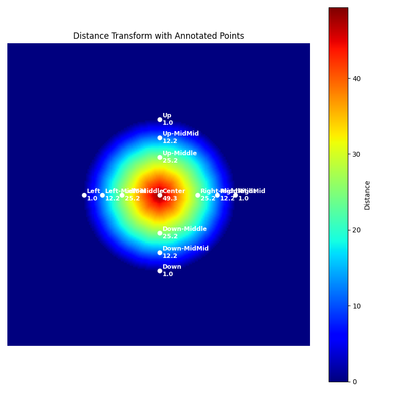
# 3. Define representative points
points = {
"Center": (100, 100),
"Up": (100, 50),
"Down": (100, 150),
"Left": (50, 100),
"Right": (150, 100),
"Up-Middle": (100, 75),
"Down-Middle": (100, 125),
"Left-Middle": (75, 100),
"Right-Middle": (125, 100),
"Up-MidMid": (100, 62),
"Down-MidMid": (100, 138),
"Left-MidMid": (62, 100),
"Right-MidMid": (138, 100),
}
# 4. Visualization
plt.figure(figsize=(8, 8))
plt.imshow(dist, cmap='jet')
plt.colorbar(label='Distance')
plt.title("Distance Transform with Annotated Points")
# 5. Annotate points
for label, (x, y) in points.items():
d = dist[y, x]
# Draw white circle marker
plt.plot(x, y, 'o', color='white', markersize=6)
# Add text label with distance value
plt.text(x + 2, y, f"{label}\n{d:.1f}", color='white',
fontsize=9, fontweight='bold', va='center')
plt.axis('off')
plt.tight_layout()
plt.show()
import cv2
import numpy as np
import matplotlib.pyplot as plt

# 1. Create a binary image with a white circle and two black square holes
img = np.zeros((200, 200), dtype=np.uint8)
cv2.circle(img, (100, 100), 70, 255, -1)  # Draw the main white circle
cv2.rectangle(img, (80, 80), (95, 95), 0, -1)    # Upper-left black hole
cv2.rectangle(img, (105, 110), (125, 130), 0, -1)  # Lower-right black hole

# 2. Apply distance transform (L2 norm)
# This computes the distance from every foreground pixel to the nearest background pixel
dist = cv2.distanceTransform(img, cv2.DIST_L2, 5)

# 3. Find the location and value of the maximum distance (deep red area)
maxVal = dist.max()
maxLoc = np.unravel_index(np.argmax(dist), dist.shape)

# 4. Define representative key points to annotate
points = {
    "Center": (100, 100),                 # Geometric center of the circle
    "MaxDist": maxLoc,                    # Point with the maximum distance from background
    "YellowArea": (100, 50),              # A mid-range distance point (yellow area)
    "OuterEdge": (100, 10),               # Near the outer edge (distance ~ 0)
    "Hole1_Center": (87, 87),             # Center of upper-left black hole
    "Hole1_Edge": (95, 95),               # Edge of upper-left hole
    "Hole2_Center": (115, 120),           # Center of lower-right black hole
    "Hole2_Edge": (105, 110),             # Edge of lower-right hole
    "X": (58, 135),                       # Custom sample point
    "Max": (128, 76),                     # Another high-value point
    "XX": (88, 112),                      # Custom sample point
}

# 5. Plot the distance transform image with annotations
plt.figure(figsize=(10, 10))
plt.imshow(dist, cmap='jet')
plt.title("Distance Transform with Annotated Key Points", fontsize=14)
plt.colorbar(label='Distance')
plt.axis('off')

# 6. Draw and annotate each key point
for label, (x, y) in points.items():
    d = dist[y, x]
    plt.plot(x, y, 'o', color='white', markersize=6)  # Mark the point
    plt.text(x + 3, y, f"{label}\n{d:.1f}", color='white', fontsize=9, fontweight='bold', va='center')

plt.tight_layout()
plt.show()
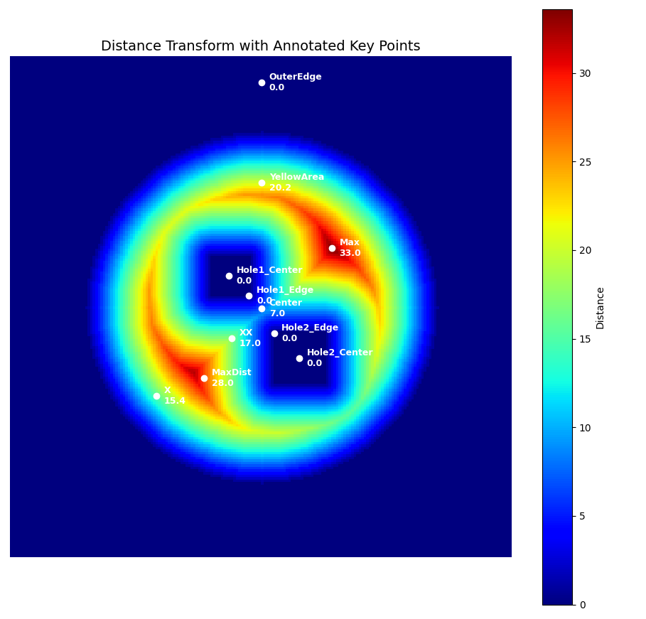
Distance Transform assigns each pixel in the foreground a value equal to its shortest distance to the nearest background pixel.
The maximum value usually appears at the center of the largest blob (here, the circle), and its location is shown as
"MaxDist"."YellowArea"and"OuterEdge"help visualize how the distance gradually decreases toward the edge."Hole1"and"Hole2"show how internal holes reset the distance to zero in those regions.